Protein-ligand complex MD Setup tutorial using BioExcel Building Blocks (biobb)
–AmberTools package version–
Based on the MDWeb Amber FULL MD Setup tutorial
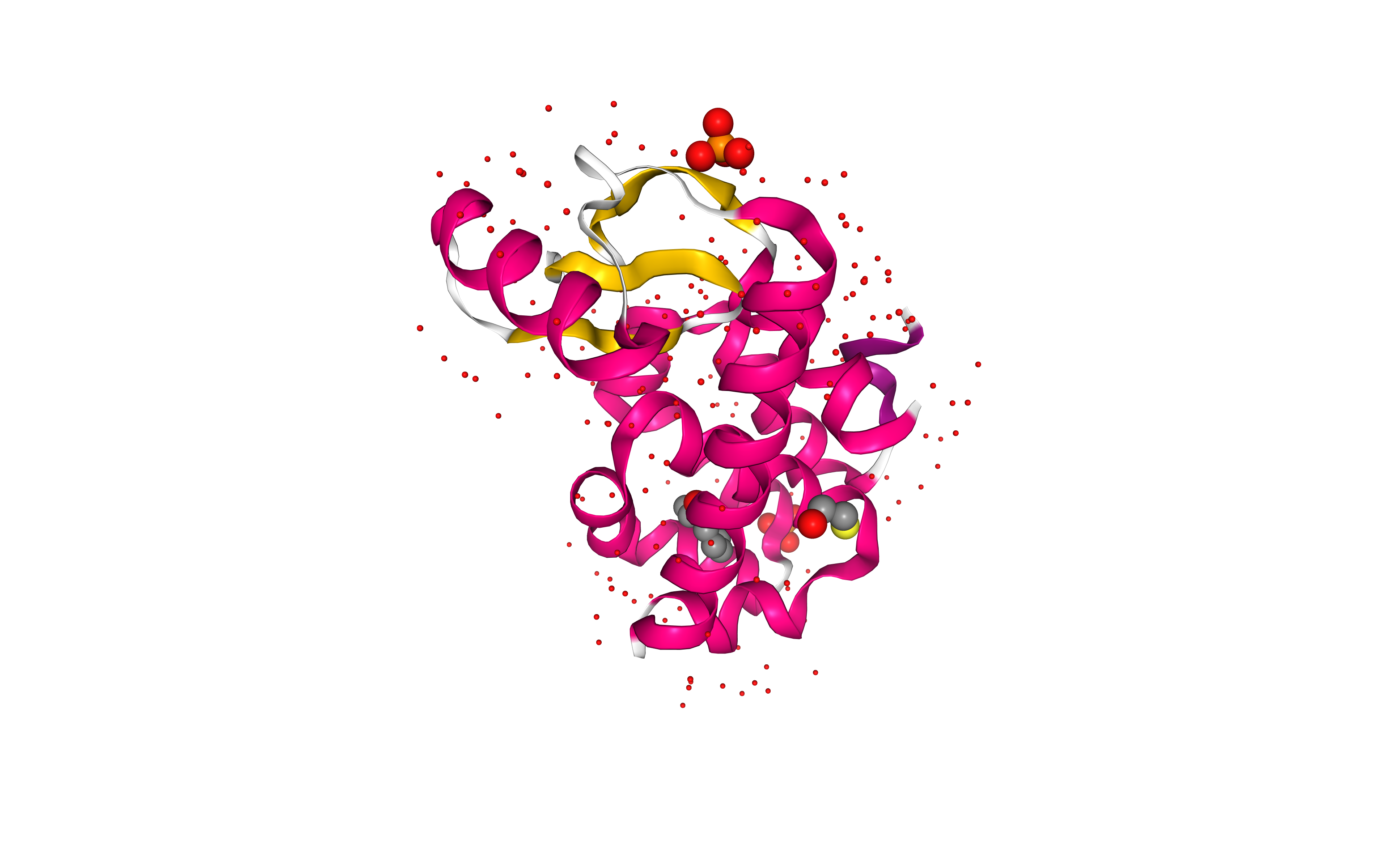
This tutorial aims to illustrate the process of setting up a simulation system containing a protein in complex with a ligand, step by step, using the BioExcel Building Blocks library (biobb) wrapping the AmberTools utility from the AMBER package. The particular example used is the T4 lysozyme protein (PDB code 3HTB, https://doi.org/10.2210/pdb3HTB/pdb) with two residue modifications L99A/M102Q complexed with the small ligand 2-propylphenol (3-letter code JZ4, https://www.rcsb.org/ligand/JZ4).
Settings
Biobb modules used
biobb_io: Tools to fetch biomolecular data from public databases.
biobb_amber: Tools to setup and run Molecular Dynamics simulations with AmberTools.
biobb_structure_utils: Tools to modify or extract information from a PDB structure file.
biobb_analysis: Tools to analyse Molecular Dynamics trajectories.
biobb_chemistry: Tools to to perform chemical conversions.
Auxiliar libraries used
jupyter: Free software, open standards, and web services for interactive computing across all programming languages.
plotly: Python interactive graphing library integrated in Jupyter notebooks.
nglview: Jupyter/IPython widget to interactively view molecular structures and trajectories in notebooks.
simpletraj: Lightweight coordinate-only trajectory reader based on code from GROMACS, MDAnalysis and VMD.
gfortran: Fortran 95/2003/2008/2018 compiler for GCC, the GNU Compiler Collection.
libgfortran5: Fortran compiler and libraries from the GNU Compiler Collection.
Conda Installation
git clone https://github.com/bioexcel/biobb_wf_amber_md_setup.git
cd biobb_wf_amber_md_setup
conda env create -f conda_env/environment.yml
conda activate biobb_AMBER_MDsetup_tutorials
jupyter-notebook biobb_wf_amber_md_setup/notebooks/mdsetup_lig/biobb_amber_complex_setup_notebook.ipynb
Pipeline steps
![]()
Input parameters
Input parameters needed:
pdbCode: PDB code of the protein structure (e.g. 3HTB, https://doi.org/10.2210/pdb3HTB/pdb)
ligandCode: 3-letter code of the ligand (e.g. JZ4, https://www.rcsb.org/ligand/JZ4)
mol_charge: Charge of the ligand (e.g. 0)
import nglview
import ipywidgets
import plotly
from plotly import subplots
import plotly.graph_objs as go

pdbCode = "3htb"
ligandCode = "JZ4"
mol_charge = 0
Fetching PDB structure
Downloading PDB structure with the protein molecule from the RCSB PDB database.
Alternatively, a PDB file can be used as starting structure.
Stripping from the downloaded structure any crystallographic water molecule or heteroatom.
Building Blocks used:
pdb from biobb_io.api.pdb
remove_pdb_water from biobb_structure_utils.utils.remove_pdb_water
remove_ligand from biobb_structure_utils.utils.remove_ligand
# Import module
from biobb_io.api.pdb import pdb

# Create properties dict and inputs/outputs
downloaded_pdb = pdbCode+'.pdb'

prop = {
    'pdb_code': pdbCode,
    'filter': False
}

#Create and launch bb
pdb(output_pdb_path=downloaded_pdb,
    properties=prop)
# Show protein
view = nglview.show_structure_file(downloaded_pdb)
view.clear_representations()
view.add_representation(repr_type='cartoon', selection='protein', color='sstruc')
view.add_representation(repr_type='ball+stick', radius='0.1', selection='water')
view.add_representation(repr_type='ball+stick', radius='0.5', selection='ligand')
view.add_representation(repr_type='ball+stick', radius='0.5', selection='ion')
view._remote_call('setSize', target='Widget', args=['','600px'])
view
# Import module
from biobb_structure_utils.utils.remove_pdb_water import remove_pdb_water

# Create properties dict and inputs/outputs
nowat_pdb = pdbCode+'.nowat.pdb'

#Create and launch bb
remove_pdb_water(input_pdb_path=downloaded_pdb,
    output_pdb_path=nowat_pdb)
# Import module
from biobb_structure_utils.utils.remove_ligand import remove_ligand

# Removing PO4 ligands:

# Create properties dict and inputs/outputs
nopo4_pdb = pdbCode+'.noPO4.pdb'

prop = {
    'ligand' : 'PO4'
}

#Create and launch bb
remove_ligand(input_structure_path=nowat_pdb,
    output_structure_path=nopo4_pdb,
    properties=prop)

# Removing BME ligand:

# Create properties dict and inputs/outputs
nobme_pdb = pdbCode+'.noBME.pdb'

prop = {
    'ligand' : 'BME'
}

#Create and launch bb
remove_ligand(input_structure_path=nopo4_pdb,
    output_structure_path=nobme_pdb,
    properties=prop)
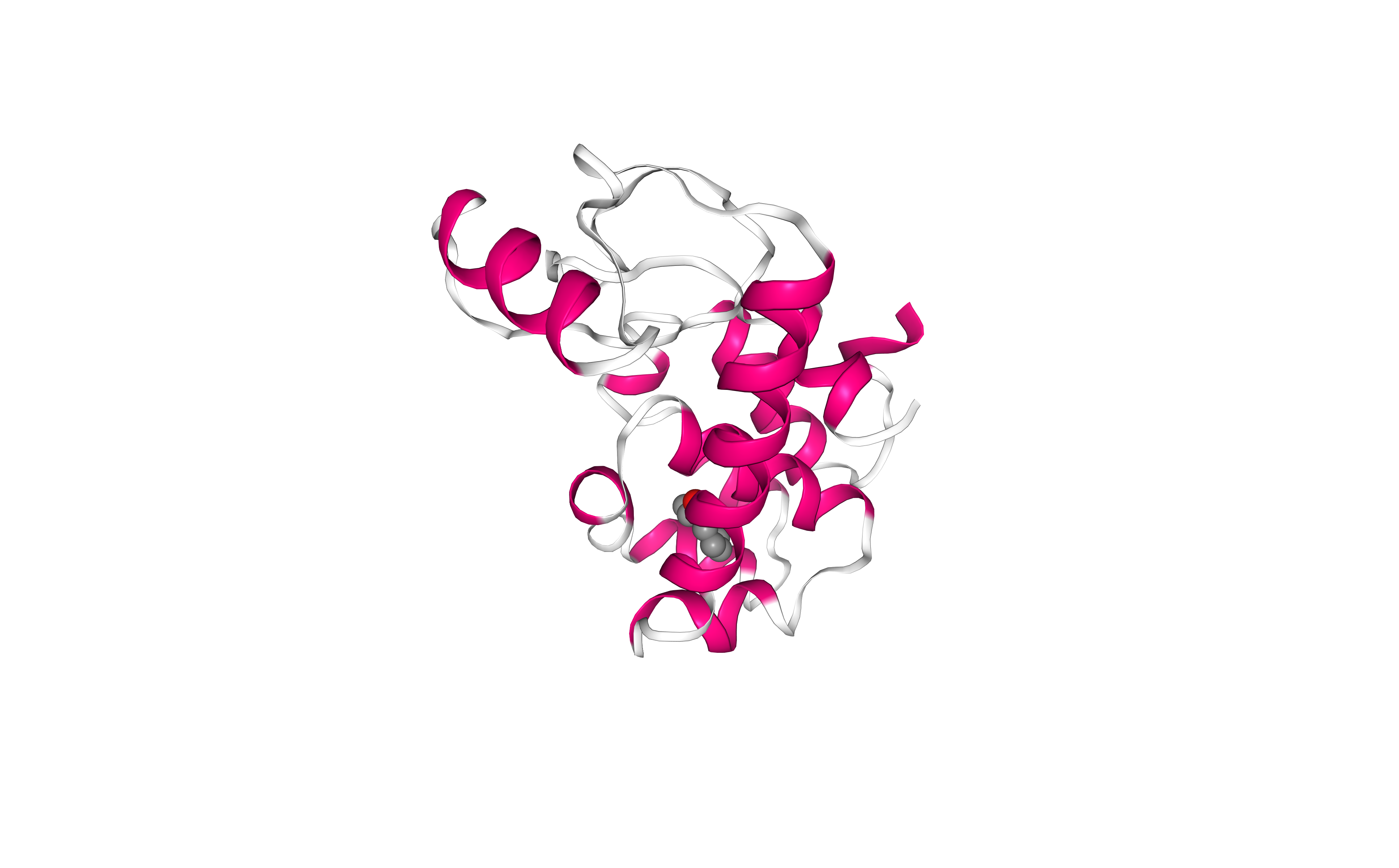
Visualizing 3D structure
# Show protein
view = nglview.show_structure_file(nobme_pdb)
view.clear_representations()
view.add_representation(repr_type='cartoon', selection='protein', color='sstruc')
view.add_representation(repr_type='ball+stick', radius='0.5', selection='hetero')
view._remote_call('setSize', target='Widget', args=['','600px'])
view
Preparing PDB file for AMBER
Before starting a protein MD setup, it is always strongly recommended to take a look at the initial structure and try to identify important properties and also possible issues. These properties and issues can be serious, as for example the definition of disulfide bridges, the presence of a non-standard aminoacids or ligands, or missing residues. Other properties and issues might not be so serious, but they still need to be addressed before starting the MD setup process. Missing hydrogen atoms, presence of alternate atomic location indicators or inserted residue codes (see PDB file format specification) are examples of these not so crucial characteristics. Please visit the AMBER tutorial: Building Protein Systems in Explicit Solvent for more examples. AmberTools utilities from AMBER MD package contain a tool able to analyse PDB files and clean them for further usage, especially with the AmberTools LEaP program: the pdb4amber tool. The next step of the workflow is running this tool to analyse our input PDB structure.
For the particular T4 Lysosyme example, the most important property that is identified by the pdb4amber utility is the presence of disulfide bridges in the structure. Those are marked changing the residue names from CYS to CYX, which is the code that AMBER force fields use to distinguish between cysteines forming or not forming disulfide bridges. This will be used in the following step to correctly form a bond between these cysteine residues.
We invite you to check what the tool does with different, more complex structures (e.g. PDB code 6N3V).
Building Blocks used:
pdb4amber_run from biobb_amber.pdb4amber.pdb4amber_run
# Import module
from biobb_amber.pdb4amber.pdb4amber_run import pdb4amber_run

# Create prop dict and inputs/outputs
output_pdb4amber_path = 'structure.pdb4amber.pdb'

# Create and launch bb
pdb4amber_run(input_pdb_path=nobme_pdb,
            output_pdb_path=output_pdb4amber_path,
            properties=prop)
Create ligand system topology
Building AMBER topology corresponding to the ligand structure.
Force field used in this tutorial step is amberGAFF: General AMBER Force Field, designed for rational drug design.
Step 1: Extract ligand structure.
Step 2: Add hydrogen atoms if missing.
Step 3: Energetically minimize the system with the new hydrogen atoms.
Step 4: Generate ligand topology (parameters).
Building Blocks used:
ExtractHeteroAtoms from biobb_structure_utils.utils.extract_heteroatoms
ReduceAddHydrogens from biobb_chemistry.ambertools.reduce_add_hydrogens
BabelMinimize from biobb_chemistry.babelm.babel_minimize
AcpypeParamsAC from biobb_chemistry.acpype.acpype_params_ac
Step 1: Extract Ligand structure
# Create Ligand system topology, STEP 1
# Extracting Ligand JZ4
# Import module
from biobb_structure_utils.utils.extract_heteroatoms import extract_heteroatoms

# Create properties dict and inputs/outputs
ligandFile = ligandCode+'.pdb'

prop = {
     'heteroatoms' : [{"name": "JZ4"}]
}

extract_heteroatoms(input_structure_path=output_pdb4amber_path,
     output_heteroatom_path=ligandFile,
     properties=prop)
Step 2: Add hydrogen atoms
# Create Ligand system topology, STEP 2
# Reduce_add_hydrogens: add Hydrogen atoms to a small molecule (using Reduce tool from Ambertools package)
# Import module
from biobb_chemistry.ambertools.reduce_add_hydrogens import reduce_add_hydrogens

# Create prop dict and inputs/outputs
output_reduce_h = ligandCode+'.reduce.H.pdb'

prop = {
    'nuclear' : 'true'
}

# Create and launch bb
reduce_add_hydrogens(input_path=ligandFile,
                   output_path=output_reduce_h,
                   properties=prop)
Step 3: Energetically minimize the system with the new hydrogen atoms.
# Create Ligand system topology, STEP 3
# Babel_minimize: Structure energy minimization of a small molecule after being modified adding hydrogen atoms
# Import module
from biobb_chemistry.babelm.babel_minimize import babel_minimize

# Create prop dict and inputs/outputs
output_babel_min = ligandCode+'.H.min.mol2'

prop = {
    'method' : 'sd',
    'criteria' : '1e-10',
    'force_field' : 'GAFF'
}


# Create and launch bb
babel_minimize(input_path=output_reduce_h,
              output_path=output_babel_min,
              properties=prop)
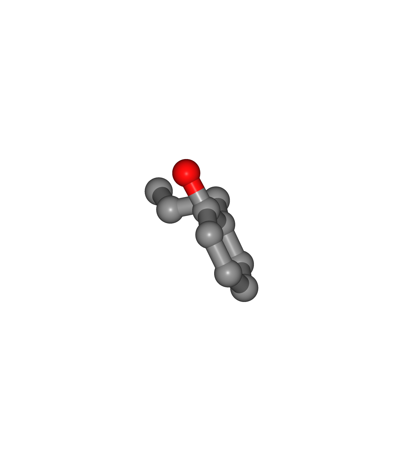
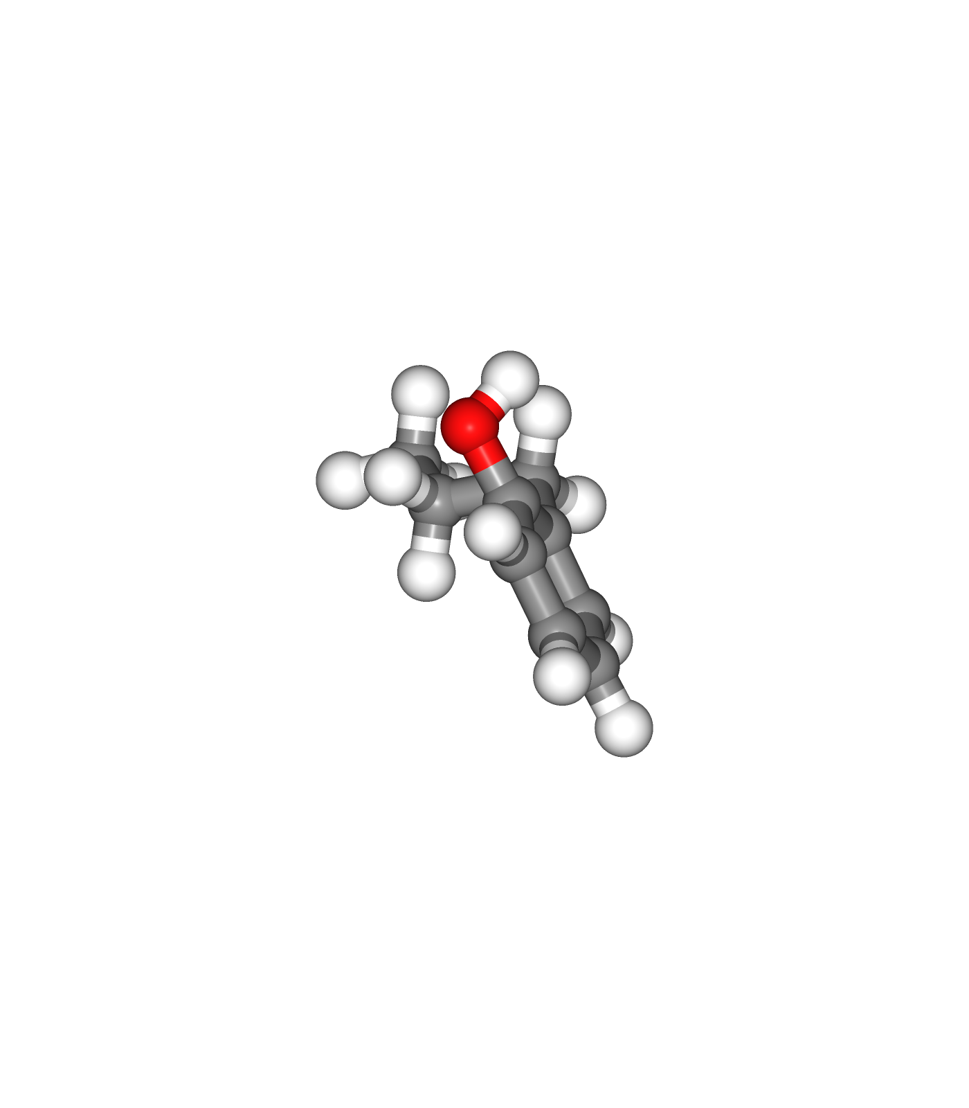
Visualizing 3D structures
Visualizing the small molecule generated PDB structures using NGL:
Original Ligand Structure (Left)
Ligand Structure with hydrogen atoms added (with Reduce program) (Center)
Ligand Structure with hydrogen atoms added (with Reduce program), energy minimized (with Open Babel) (Right)
# Show different structures generated (for comparison)

view1 = nglview.show_structure_file(ligandFile)
view1.add_representation(repr_type='ball+stick')
view1._remote_call('setSize', target='Widget', args=['350px','400px'])
view1.camera='orthographic'
view1
view2 = nglview.show_structure_file(output_reduce_h)
view2.add_representation(repr_type='ball+stick')
view2._remote_call('setSize', target='Widget', args=['350px','400px'])
view2.camera='orthographic'
view2
view3 = nglview.show_structure_file(output_babel_min)
view3.add_representation(repr_type='ball+stick')
view3._remote_call('setSize', target='Widget', args=['350px','400px'])
view3.camera='orthographic'
view3
ipywidgets.HBox([view1, view2, view3])

### Step 4: Generate ligand topology (parameters).
# Create Ligand system topology, STEP 4
# Acpype_params_gmx: Generation of topologies for AMBER with ACPype
# Import module
from biobb_chemistry.acpype.acpype_params_ac import acpype_params_ac

# Create prop dict and inputs/outputs
output_acpype_inpcrd = ligandCode+'params.inpcrd'
output_acpype_frcmod = ligandCode+'params.frcmod'
output_acpype_lib = ligandCode+'params.lib'
output_acpype_prmtop = ligandCode+'params.prmtop'
output_acpype = ligandCode+'params'

prop = {
    'basename' : output_acpype,
    'charge' : mol_charge
}

# Create and launch bb
acpype_params_ac(input_path=output_babel_min,
                output_path_inpcrd=output_acpype_inpcrd,
                output_path_frcmod=output_acpype_frcmod,
                output_path_lib=output_acpype_lib,
                output_path_prmtop=output_acpype_prmtop,
                properties=prop)
Create protein-ligand complex system topology
Building AMBER topology corresponding to the protein-ligand complex structure.
IMPORTANT: the previous pdb4amber building block is changing the proper cysteines residue naming in the PDB file from CYS to CYX so that this step can automatically identify and add the disulfide bonds to the system topology.
The force field used in this tutorial is ff14SB for the protein, an evolution of the ff99SB force field with improved accuracy of protein side chains and backbone parameters; and the gaff force field for the small molecule. Water molecules type used in this tutorial is tip3p.
Adding side chain atoms and hydrogen atoms if missing. Forming disulfide bridges according to the info added in the previous step.
NOTE: From this point on, the protein-ligand complex structure and topology generated can be used in a regular MD setup.
Generating three output files:
AMBER structure (PDB file)
AMBER topology (AMBER Parmtop file)
AMBER coordinates (AMBER Coordinate/Restart file)
Building Blocks used:
leap_gen_top from biobb_amber.leap.leap_gen_top
# Import module
from biobb_amber.leap.leap_gen_top import leap_gen_top

# Create prop dict and inputs/outputs
output_pdb_path = 'structure.leap.pdb'
output_top_path = 'structure.leap.top'
output_crd_path = 'structure.leap.crd'

prop = {
    "forcefield" : ["protein.ff14SB","gaff"]
}

# Create and launch bb
leap_gen_top(input_pdb_path=output_pdb4amber_path,
           input_lib_path=output_acpype_lib,
           input_frcmod_path=output_acpype_frcmod,
           output_pdb_path=output_pdb_path,
           output_top_path=output_top_path,
           output_crd_path=output_crd_path,
           properties=prop)
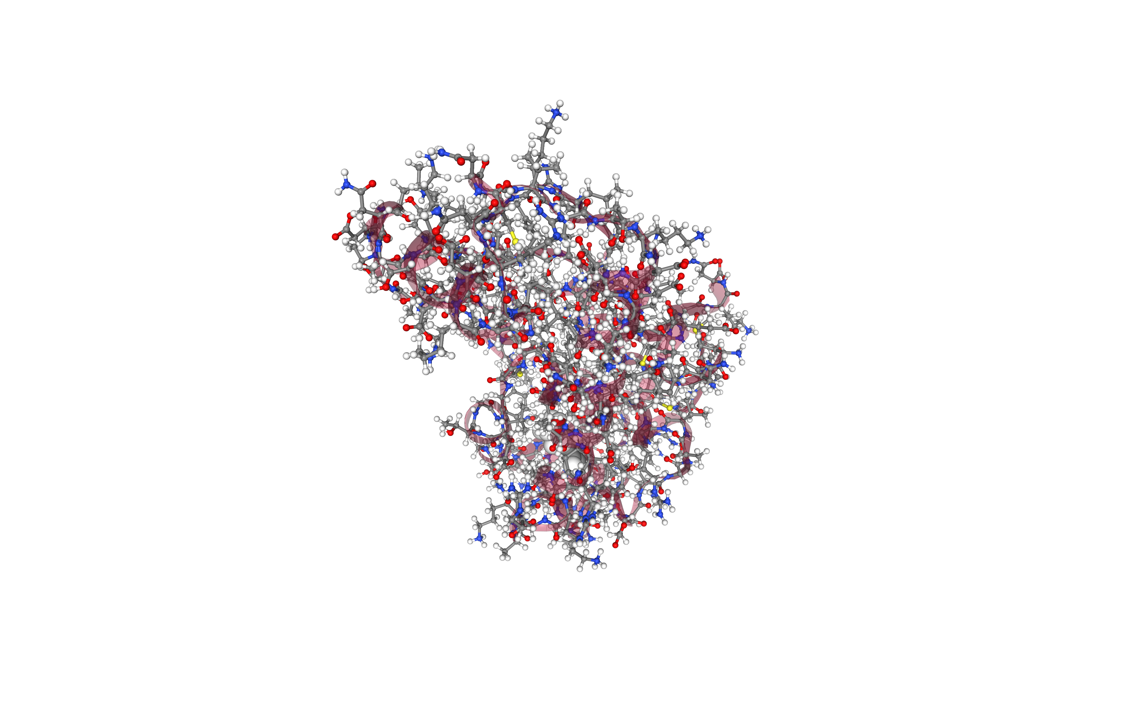
Visualizing 3D structure
Visualizing the PDB structure using NGL.
Try to identify the differences between the structure generated for the system topology and the original one (e.g. hydrogen atoms).
import nglview
import ipywidgets

# Show protein
view = nglview.show_structure_file(output_pdb_path)
view.clear_representations()
view.add_representation(repr_type='cartoon', selection='protein', opacity='0.4')
view.add_representation(repr_type='ball+stick', selection='protein')
view.add_representation(repr_type='ball+stick', radius='0.5', selection='JZ4')
view._remote_call('setSize', target='Widget', args=['','600px'])
view
Energetically minimize the structure
Energetically minimize the protein-ligand complex structure (in vacuo) using the sander tool from the AMBER MD package. This step is relaxing the structure, usually constrained, especially when coming from an X-ray crystal structure.
The miminization process is done in two steps:
Step 1: Hydrogen minimization, applying position restraints (50 Kcal/mol.$Å^{2}$) to the protein heavy atoms.
Step 2: System minimization, with no restraints.
Building Blocks used:
sander_mdrun from biobb_amber.sander.sander_mdrun
process_minout from biobb_amber.process.process_minout
Step 1: Minimize Hydrogens
Hydrogen minimization, applying position restraints (50 Kcal/mol.$Å^{2}$) to the protein heavy atoms.
# Import module
from biobb_amber.sander.sander_mdrun import sander_mdrun

# Create prop dict and inputs/outputs
output_h_min_traj_path = 'sander.h_min.x'
output_h_min_rst_path = 'sander.h_min.rst'
output_h_min_log_path = 'sander.h_min.log'

prop = {
    'simulation_type' : "min_vacuo",
    "mdin" : {
        'maxcyc' : 500,
        'ntpr' : 5,
        'ntr' : 1,
        'restraintmask' : '\":*&!@H=\"',
        'restraint_wt' : 50.0
    }
}

# Create and launch bb
sander_mdrun(input_top_path=output_top_path,
            input_crd_path=output_crd_path,
            input_ref_path=output_crd_path,
            output_traj_path=output_h_min_traj_path,
            output_rst_path=output_h_min_rst_path,
            output_log_path=output_h_min_log_path,
            properties=prop)
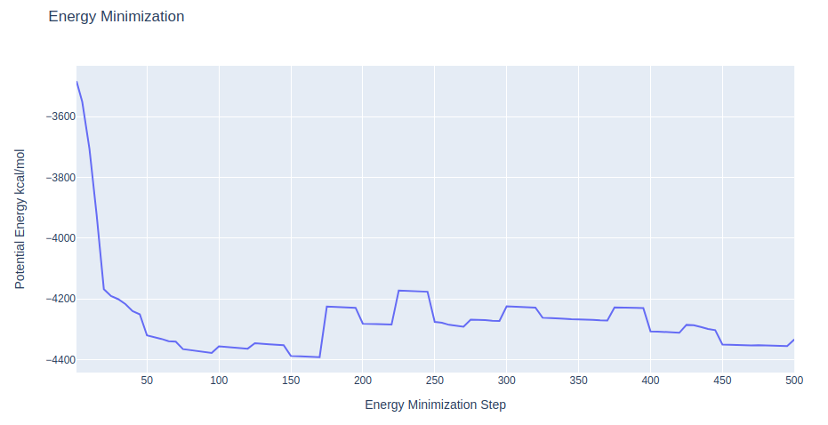
Checking Energy Minimization results
Checking energy minimization results. Plotting potential energy along time during the minimization process.
# Import module
from biobb_amber.process.process_minout import process_minout

# Create prop dict and inputs/outputs
output_h_min_dat_path = 'sander.h_min.energy.dat'

prop = {
    "terms" : ['ENERGY']
}

# Create and launch bb
process_minout(input_log_path=output_h_min_log_path,
            output_dat_path=output_h_min_dat_path,
            properties=prop)
with open(output_h_min_dat_path,'r') as energy_file:
    x,y = map(
        list,
        zip(*[
            (float(line.split()[0]),float(line.split()[1]))
            for line in energy_file
            if not line.startswith(("#","@"))
            if float(line.split()[1]) < 1000
        ])
    )

plotly.offline.init_notebook_mode(connected=True)

fig = {
    "data": [go.Scatter(x=x, y=y)],
    "layout": go.Layout(title="Energy Minimization",
                        xaxis=dict(title = "Energy Minimization Step"),
                        yaxis=dict(title = "Potential Energy kcal/mol")
                       )
}

plotly.offline.iplot(fig)
Step 2: Minimize the system
System minimization, with restraints only on the small molecule, to avoid a possible change in position due to protein repulsion.
# Import module
from biobb_amber.sander.sander_mdrun import sander_mdrun

# Create prop dict and inputs/outputs
output_n_min_traj_path = 'sander.n_min.x'
output_n_min_rst_path = 'sander.n_min.rst'
output_n_min_log_path = 'sander.n_min.log'

prop = {
    'simulation_type' : "min_vacuo",
    "mdin" : {
        'maxcyc' : 500,
        'ntpr' : 5,
        'restraintmask' : '\":' + ligandCode + '\"',
        'restraint_wt' : 500.0
    }
}

# Create and launch bb
sander_mdrun(input_top_path=output_top_path,
            input_crd_path=output_h_min_rst_path,
            output_traj_path=output_n_min_traj_path,
            output_rst_path=output_n_min_rst_path,
            output_log_path=output_n_min_log_path,
            properties=prop)
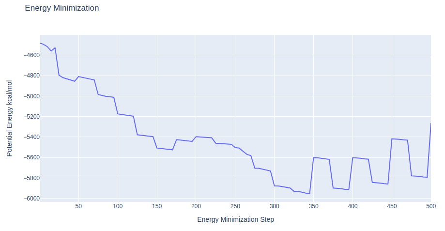
Checking Energy Minimization results
Checking energy minimization results. Plotting potential energy by time during the minimization process.
# Import module
from biobb_amber.process.process_minout import process_minout

# Create prop dict and inputs/outputs
output_n_min_dat_path = 'sander.n_min.energy.dat'

prop = {
    "terms" : ['ENERGY']
}

# Create and launch bb
process_minout(input_log_path=output_n_min_log_path,
            output_dat_path=output_n_min_dat_path,
            properties=prop)
with open(output_n_min_dat_path,'r') as energy_file:
    x,y = map(
        list,
        zip(*[
            (float(line.split()[0]),float(line.split()[1]))
            for line in energy_file
            if not line.startswith(("#","@"))
            if float(line.split()[1]) < 1000
        ])
    )

plotly.offline.init_notebook_mode(connected=True)

fig = {
    "data": [go.Scatter(x=x, y=y)],
    "layout": go.Layout(title="Energy Minimization",
                        xaxis=dict(title = "Energy Minimization Step"),
                        yaxis=dict(title = "Potential Energy kcal/mol")
                       )
}

plotly.offline.iplot(fig)
Create solvent box and solvating the system
Define the unit cell for the protein structure MD system to fill it with water molecules.
A truncated octahedron box is used to define the unit cell, with a distance from the protein to the box edge of 9.0 Angstroms.
The solvent type used is the default TIP3P water model, a generic 3-point solvent model.
Building Blocks used:
amber_to_pdb from biobb_amber.ambpdb.amber_to_pdb
leap_solvate from biobb_amber.leap.leap_solvate
Getting minimized structure
Getting the result of the energetic minimization and converting it to PDB format to be then used as input for the water box generation.
This is achieved by converting from AMBER topology + coordinates files to a PDB file using the ambpdb tool from the AMBER MD package.
# Import module
from biobb_amber.ambpdb.amber_to_pdb import amber_to_pdb

# Create prop dict and inputs/outputs
output_ambpdb_path = 'structure.ambpdb.pdb'

# Create and launch bb
amber_to_pdb(input_top_path=output_top_path,
            input_crd_path=output_n_min_rst_path,
            output_pdb_path=output_ambpdb_path)
Create water box
Define the unit cell for the protein-ligand complex structure MD system and fill it with water molecules.
# Import module
from biobb_amber.leap.leap_solvate import leap_solvate

# Create prop dict and inputs/outputs
output_solv_pdb_path = 'structure.solv.pdb'
output_solv_top_path = 'structure.solv.parmtop'
output_solv_crd_path = 'structure.solv.crd'

prop = {
    "forcefield" : ["protein.ff14SB","gaff"],
    "water_type": "TIP3PBOX",
    "distance_to_molecule": "9.0",
    "box_type": "truncated_octahedron"
}

# Create and launch bb
leap_solvate(input_pdb_path=output_ambpdb_path,
             input_lib_path=output_acpype_lib,
             input_frcmod_path=output_acpype_frcmod,
             output_pdb_path=output_solv_pdb_path,
             output_top_path=output_solv_top_path,
             output_crd_path=output_solv_crd_path,
             properties=prop)
Adding ions
Neutralizing the system and adding an additional ionic concentration using the leap tool from the AMBER MD package.
Using Sodium (Na+) and Chloride (Cl-) counterions and an additional ionic concentration of 150mM.
Building Blocks used:
leap_add_ions from biobb_amber.leap.leap_add_ions
# Import module
from biobb_amber.leap.leap_add_ions import leap_add_ions

# Create prop dict and inputs/outputs
output_ions_pdb_path = 'structure.ions.pdb'
output_ions_top_path = 'structure.ions.parmtop'
output_ions_crd_path = 'structure.ions.crd'

prop = {
    "forcefield" : ["protein.ff14SB","gaff"],
    "neutralise" : True,
    "positive_ions_type": "Na+",
    "negative_ions_type": "Cl-",
    "ionic_concentration" : 150, # 150mM
    "box_type": "truncated_octahedron"
}

# Create and launch bb
leap_add_ions(input_pdb_path=output_solv_pdb_path,
            input_lib_path=output_acpype_lib,
            input_frcmod_path=output_acpype_frcmod,
           output_pdb_path=output_ions_pdb_path,
           output_top_path=output_ions_top_path,
           output_crd_path=output_ions_crd_path,
           properties=prop)
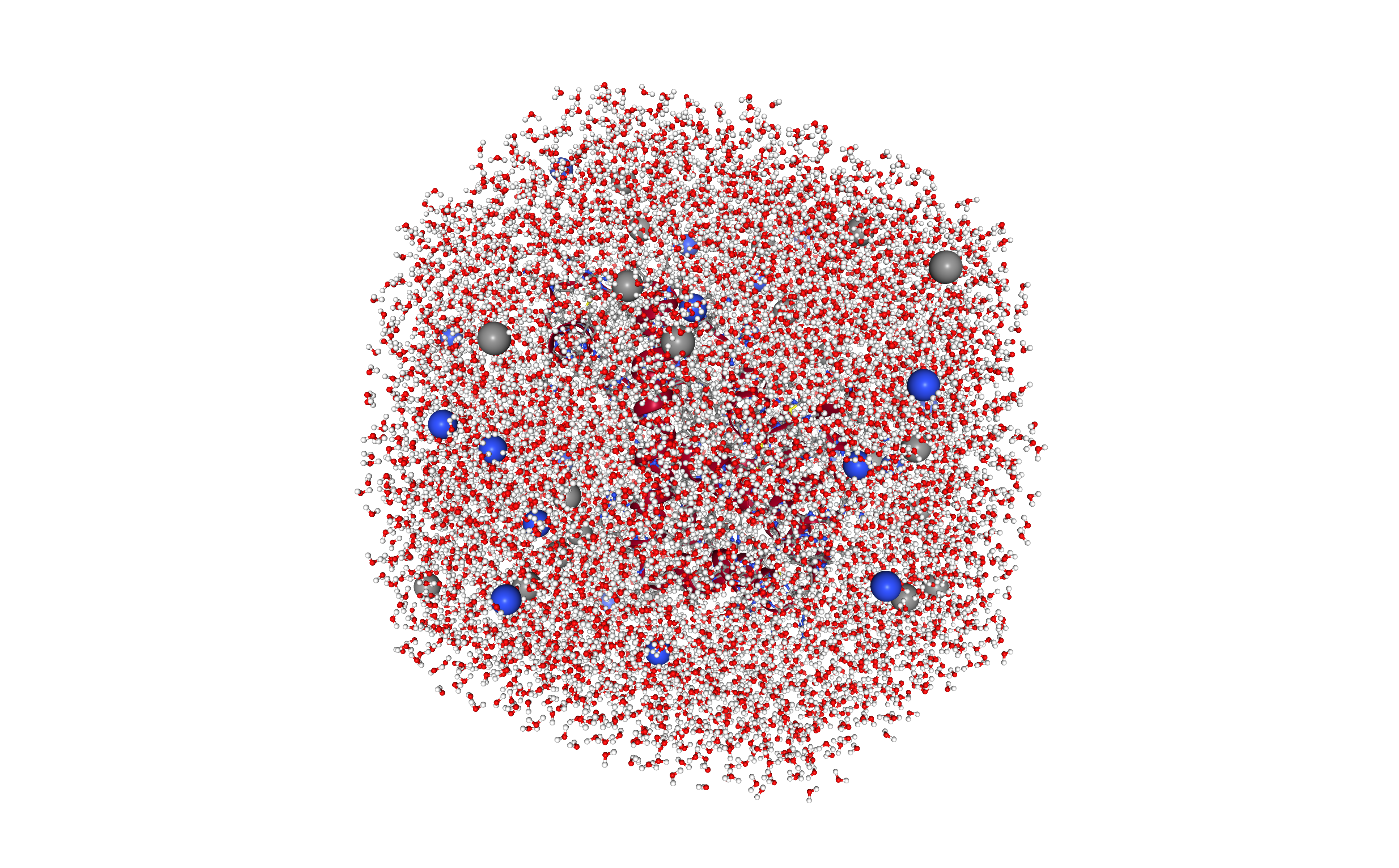
Visualizing 3D structure
Visualizing the protein-ligand complex system with the newly added solvent box and counterions using NGL.
Note the truncated octahedron box filled with water molecules surrounding the protein structure, as well as the randomly placed positive (Na+, blue) and negative (Cl-, gray) counterions.
# Show protein
view = nglview.show_structure_file(output_ions_pdb_path)
view.clear_representations()
view.add_representation(repr_type='cartoon', selection='protein')
view.add_representation(repr_type='ball+stick', selection='solvent')
view.add_representation(repr_type='spacefill', selection='Cl- Na+')
view._remote_call('setSize', target='Widget', args=['','600px'])
view
Energetically minimize the system
Energetically minimize the system (protein structure + ligand + solvent + ions) using the sander tool from the AMBER MD package. Restraining heavy atoms with a force constant of 15 15 Kcal/mol.$Å^{2}$ to their initial positions.
Step 1: Energetically minimize the system through 500 minimization cycles.
Step 2: Checking energy minimization results. Plotting energy by time during the minimization process.
Building Blocks used:
sander_mdrun from biobb_amber.sander.sander_mdrun
process_minout from biobb_amber.process.process_minout
Step 1: Running Energy Minimization
The minimization type of the simulation_type property contains the main default parameters to run an energy minimization:
imin = 1 ; Minimization flag, perform an energy minimization.
maxcyc = 500; The maximum number of cycles of minimization.
ntb = 1; Periodic boundaries: constant volume.
ntmin = 2; Minimization method: steepest descent.
In this particular example, the method used to run the energy minimization is the default steepest descent, with a maximum number of 500 cycles and periodic conditions.
# Import module
from biobb_amber.sander.sander_mdrun import sander_mdrun

# Create prop dict and inputs/outputs
output_min_traj_path = 'sander.min.x'
output_min_rst_path = 'sander.min.rst'
output_min_log_path = 'sander.min.log'

prop = {
    "simulation_type" : "minimization",
    "mdin" : {
        'maxcyc' : 300, # Reducing the number of minimization steps for the sake of time
        'ntr' : 1,      # Overwritting restrain parameter
        'restraintmask' : '\"!:WAT,Cl-,Na+\"',      # Restraining solute
        'restraint_wt' : 15.0                       # With a force constant of 50 Kcal/mol*A2
    }
}

# Create and launch bb
sander_mdrun(input_top_path=output_ions_top_path,
            input_crd_path=output_ions_crd_path,
            input_ref_path=output_ions_crd_path,
            output_traj_path=output_min_traj_path,
            output_rst_path=output_min_rst_path,
            output_log_path=output_min_log_path,
            properties=prop)
Step 2: Checking Energy Minimization results
Checking energy minimization results. Plotting potential energy along time during the minimization process.
# Import module
from biobb_amber.process.process_minout import process_minout

# Create prop dict and inputs/outputs
output_dat_path = 'sander.min.energy.dat'

prop = {
    "terms" : ['ENERGY']
}

# Create and launch bb
process_minout(input_log_path=output_min_log_path,
            output_dat_path=output_dat_path,
            properties=prop)
with open(output_dat_path,'r') as energy_file:
    x,y = map(
        list,
        zip(*[
            (float(line.split()[0]),float(line.split()[1]))
            for line in energy_file
            if not line.startswith(("#","@"))
            if float(line.split()[1]) < 1000
        ])
    )

plotly.offline.init_notebook_mode(connected=True)

fig = {
    "data": [go.Scatter(x=x, y=y)],
    "layout": go.Layout(title="Energy Minimization",
                        xaxis=dict(title = "Energy Minimization Step"),
                        yaxis=dict(title = "Potential Energy kcal/mol")
                       )
}

plotly.offline.iplot(fig)
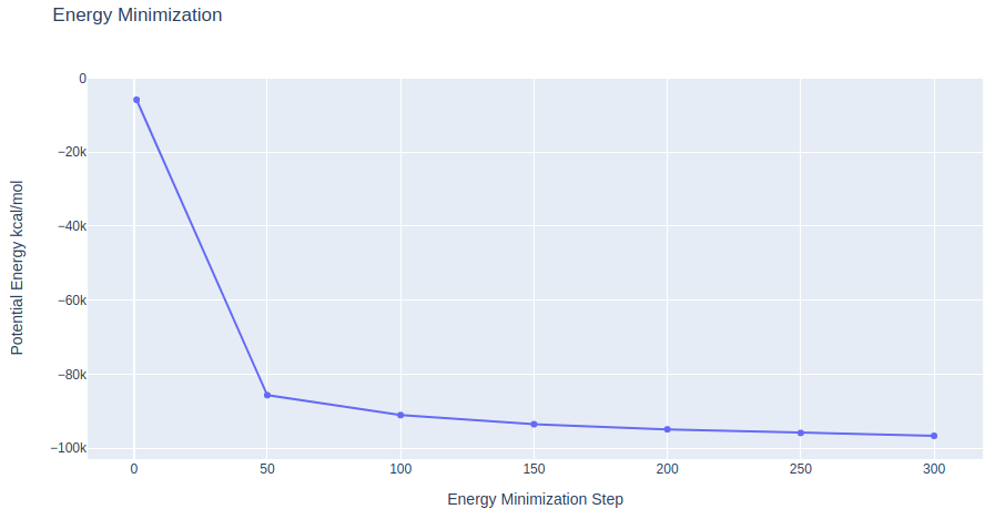
Heating the system
Warming up the prepared system using the sander tool from the AMBER MD package. Going from 0 to the desired temperature, in this particular example, 300K. Solute atoms restrained (force constant of 10 Kcal/mol). Length 5ps.
Step 1: Warming up the system through 500 MD steps.
Step 2: Checking results for the system warming up. Plotting temperature along time during the heating process.
Building Blocks used:
sander_mdrun from biobb_amber.sander.sander_mdrun
process_mdout from biobb_amber.process.process_mdout
Step 1: Warming up the system
The heat type of the simulation_type property contains the main default parameters to run a system warming up:
imin = 0; Run MD (no minimization)
ntx = 5; Read initial coords and vels from restart file
cut = 10.0; Cutoff for non bonded interactions in Angstroms
ntr = 0; No restrained atoms
ntc = 2; SHAKE for constraining length of bonds involving Hydrogen atoms
ntf = 2; Bond interactions involving H omitted
ntt = 3; Constant temperature using Langevin dynamics
ig = -1; Seed for pseudo-random number generator
ioutfm = 1; Write trajectory in netcdf format
iwrap = 1; Wrap coords into primary box
nstlim = 5000; Number of MD steps
dt = 0.002; Time step (in ps)
tempi = 0.0; Initial temperature (0 K)
temp0 = 300.0; Final temperature (300 K)
irest = 0; No restart from previous simulation
ntb = 1; Periodic boundary conditions at constant volume
gamma_ln = 1.0; Collision frequency for Langevin dynamics (in 1/ps)
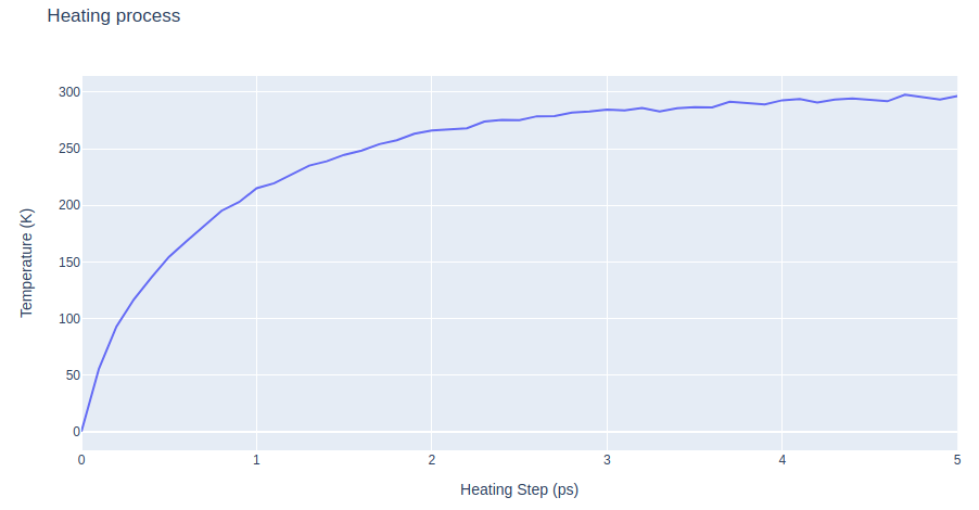
In this particular example, the heating of the system is done in 2500 steps (5ps) and is going from 0K to 300K (note that the number of steps has been reduced in this tutorial, for the sake of time).
# Import module
from biobb_amber.sander.sander_mdrun import sander_mdrun

# Create prop dict and inputs/outputs
output_heat_traj_path = 'sander.heat.netcdf'
output_heat_rst_path = 'sander.heat.rst'
output_heat_log_path = 'sander.heat.log'

prop = {
    "simulation_type" : "heat",
    "mdin" : {
        'nstlim' : 2500, # Reducing the number of steps for the sake of time (5ps)
        'ntr' : 1,     # Overwritting restrain parameter
        'restraintmask' : '\"!:WAT,Cl-,Na+\"',      # Restraining solute
        'restraint_wt' : 10.0                       # With a force constant of 10 Kcal/mol*A2
    }
}

# Create and launch bb
sander_mdrun(input_top_path=output_ions_top_path,
            input_crd_path=output_min_rst_path,
            input_ref_path=output_min_rst_path,
            output_traj_path=output_heat_traj_path,
            output_rst_path=output_heat_rst_path,
            output_log_path=output_heat_log_path,
            properties=prop)
Step 2: Checking results from the system warming up
Checking system warming up output. Plotting temperature along time during the heating process.
# Import module
from biobb_amber.process.process_mdout import process_mdout

# Create prop dict and inputs/outputs
output_dat_heat_path = 'sander.md.temp.dat'

prop = {
    "terms" : ['TEMP']
}

# Create and launch bb
process_mdout(input_log_path=output_heat_log_path,
            output_dat_path=output_dat_heat_path,
            properties=prop)
with open(output_dat_heat_path,'r') as energy_file:
    x,y = map(
        list,
        zip(*[
            (float(line.split()[0]),float(line.split()[1]))
            for line in energy_file
            if not line.startswith(("#","@"))
            if float(line.split()[1]) < 1000
        ])
    )

plotly.offline.init_notebook_mode(connected=True)

fig = {
    "data": [go.Scatter(x=x, y=y)],
    "layout": go.Layout(title="Heating process",
                        xaxis=dict(title = "Heating Step (ps)"),
                        yaxis=dict(title = "Temperature (K)")
                       )
}

plotly.offline.iplot(fig)
Equilibrate the system (NVT)
Equilibrate the protein-ligand complex system in NVT ensemble (constant Number of particles, Volume and Temperature). Protein heavy atoms will be restrained using position restraining forces: movement is permitted, but only after overcoming a substantial energy penalty. The utility of position restraints is that they allow us to equilibrate our solvent around our protein, without the added variable of structural changes in the protein.
Step 1: Equilibrate the protein system with NVT ensemble.
Step 2: Checking NVT Equilibration results. Plotting system temperature by time during the NVT equilibration process.
Building Blocks used:
sander_mdrun from biobb_amber.sander.sander_mdrun
process_mdout from biobb_amber.process.process_mdout
Step 1: Equilibrating the system (NVT)
The nvt type of the simulation_type property contains the main default parameters to run a system equilibration in NVT ensemble:
imin = 0; Run MD (no minimization)
ntx = 5; Read initial coords and vels from restart file
cut = 10.0; Cutoff for non bonded interactions in Angstroms
ntr = 0; No restrained atoms
ntc = 2; SHAKE for constraining length of bonds involving Hydrogen atoms
ntf = 2; Bond interactions involving H omitted
ntt = 3; Constant temperature using Langevin dynamics
ig = -1; Seed for pseudo-random number generator
ioutfm = 1; Write trajectory in netcdf format
iwrap = 1; Wrap coords into primary box
nstlim = 5000; Number of MD steps
dt = 0.002; Time step (in ps)
irest = 1; Restart previous simulation
ntb = 1; Periodic boundary conditions at constant volume
gamma_ln = 5.0; Collision frequency for Langevin dynamics (in 1/ps)
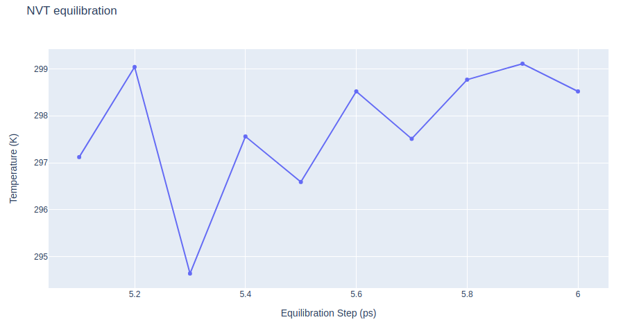
In this particular example, the NVT equilibration of the system is done in 500 steps (note that the number of steps has been reduced in this tutorial, for the sake of time).
# Import module
from biobb_amber.sander.sander_mdrun import sander_mdrun

# Create prop dict and inputs/outputs
output_nvt_traj_path = 'sander.nvt.netcdf'
output_nvt_rst_path = 'sander.nvt.rst'
output_nvt_log_path = 'sander.nvt.log'

prop = {
    "simulation_type" : 'nvt',
    "mdin" : {
        'nstlim' : 500, # Reducing the number of steps for the sake of time (1ps)
        'ntr' : 1,     # Overwritting restrain parameter
        'restraintmask' : '\"!:WAT,Cl-,Na+ & !@H=\"',      # Restraining solute heavy atoms
        'restraint_wt' : 5.0                              # With a force constant of 5 Kcal/mol*A2
    }
}

# Create and launch bb
sander_mdrun(input_top_path=output_ions_top_path,
            input_crd_path=output_heat_rst_path,
            input_ref_path=output_heat_rst_path,
            output_traj_path=output_nvt_traj_path,
            output_rst_path=output_nvt_rst_path,
            output_log_path=output_nvt_log_path,
            properties=prop)
Step 2: Checking NVT Equilibration results
Checking NVT Equilibration results. Plotting system temperature by time during the NVT equilibration process.
# Import module
from biobb_amber.process.process_mdout import process_mdout

# Create prop dict and inputs/outputs
output_dat_nvt_path = 'sander.md.nvt.temp.dat'

prop = {
    "terms" : ['TEMP']
}

# Create and launch bb
process_mdout(input_log_path=output_nvt_log_path,
            output_dat_path=output_dat_nvt_path,
            properties=prop)
with open(output_dat_nvt_path,'r') as energy_file:
    x,y = map(
        list,
        zip(*[
            (float(line.split()[0]),float(line.split()[1]))
            for line in energy_file
            if not line.startswith(("#","@"))
            if float(line.split()[1]) < 1000
        ])
    )

plotly.offline.init_notebook_mode(connected=True)

fig = {
    "data": [go.Scatter(x=x, y=y)],
    "layout": go.Layout(title="NVT equilibration",
                        xaxis=dict(title = "Equilibration Step (ps)"),
                        yaxis=dict(title = "Temperature (K)")
                       )
}

plotly.offline.iplot(fig)
Equilibrate the system (NPT)
Equilibrate the protein-ligand complex system in NPT ensemble (constant Number of particles, Pressure and Temperature). Protein heavy atoms will be restrained using position restraining forces: movement is permitted, but only after overcoming a substantial energy penalty. The utility of position restraints is that they allow us to equilibrate our solvent around our protein, without the added variable of structural changes in the protein.
Step 1: Equilibrate the protein system with NPT ensemble.
Step 2: Checking NPT Equilibration results. Plotting system pressure and density by time during the NVT equilibration process.
Building Blocks used:
sander_mdrun from biobb_amber.sander.sander_mdrun
process_mdout from biobb_amber.process.process_mdout
Step 1: Equilibrating the system (NPT)
The npt type of the simulation_type property contains the main default parameters to run a system equilibration in NPT ensemble:
imin = 0; Run MD (no minimization)
ntx = 5; Read initial coords and vels from restart file
cut = 10.0; Cutoff for non bonded interactions in Angstroms
ntr = 0; No restrained atoms
ntc = 2; SHAKE for constraining length of bonds involving Hydrogen atoms
ntf = 2; Bond interactions involving H omitted
ntt = 3; Constant temperature using Langevin dynamics
ig = -1; Seed for pseudo-random number generator
ioutfm = 1; Write trajectory in netcdf format
iwrap = 1; Wrap coords into primary box
nstlim = 5000; Number of MD steps
dt = 0.002; Time step (in ps)
irest = 1; Restart previous simulation
gamma_ln = 5.0; Collision frequency for Langevin dynamics (in 1/ps)
pres0 = 1.0; Reference pressure
ntp = 1; Constant pressure dynamics: md with isotropic position scaling
taup = 2.0; Pressure relaxation time (in ps)
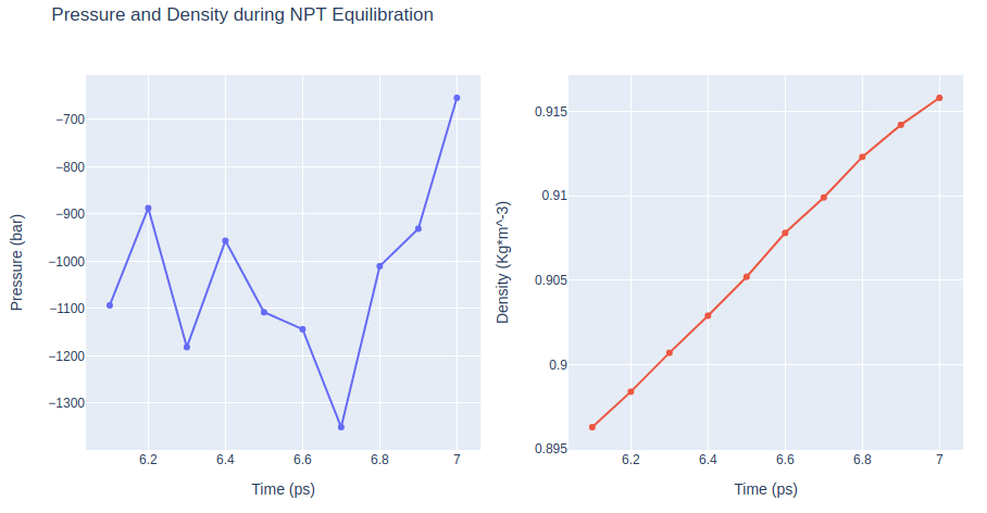
In this particular example, the NPT equilibration of the system is done in 500 steps (note that the number of steps has been reduced in this tutorial, for the sake of time).
# Import module
from biobb_amber.sander.sander_mdrun import sander_mdrun

# Create prop dict and inputs/outputs
output_npt_traj_path = 'sander.npt.netcdf'
output_npt_rst_path = 'sander.npt.rst'
output_npt_log_path = 'sander.npt.log'

prop = {
    "simulation_type" : 'npt',
    "mdin" : {
        'nstlim' : 500, # Reducing the number of steps for the sake of time (1ps)
        'ntr' : 1,     # Overwritting restrain parameter
        'restraintmask' : '\"!:WAT,Cl-,Na+ & !@H=\"',      # Restraining solute heavy atoms
        'restraint_wt' : 2.5                               # With a force constant of 2.5 Kcal/mol*A2
    }
}

# Create and launch bb
sander_mdrun(input_top_path=output_ions_top_path,
            input_crd_path=output_nvt_rst_path,
            input_ref_path=output_nvt_rst_path,
            output_traj_path=output_npt_traj_path,
            output_rst_path=output_npt_rst_path,
            output_log_path=output_npt_log_path,
            properties=prop)
Step 2: Checking NPT Equilibration results
Checking NPT Equilibration results. Plotting system pressure and density by time during the NPT equilibration process.
# Import module
from biobb_amber.process.process_mdout import process_mdout

# Create prop dict and inputs/outputs
output_dat_npt_path = 'sander.md.npt.dat'

prop = {
    "terms" : ['PRES','DENSITY']
}

# Create and launch bb
process_mdout(input_log_path=output_npt_log_path,
            output_dat_path=output_dat_npt_path,
            properties=prop)
# Read pressure and density data from file
with open(output_dat_npt_path,'r') as pd_file:
    x,y,z = map(
        list,
        zip(*[
            (float(line.split()[0]),float(line.split()[1]),float(line.split()[2]))
            for line in pd_file
            if not line.startswith(("#","@"))
        ])
    )

plotly.offline.init_notebook_mode(connected=True)

trace1 = go.Scatter(
    x=x,y=y
)
trace2 = go.Scatter(
    x=x,y=z
)

fig = subplots.make_subplots(rows=1, cols=2, print_grid=False)

fig.append_trace(trace1, 1, 1)
fig.append_trace(trace2, 1, 2)

fig['layout']['xaxis1'].update(title='Time (ps)')
fig['layout']['xaxis2'].update(title='Time (ps)')
fig['layout']['yaxis1'].update(title='Pressure (bar)')
fig['layout']['yaxis2'].update(title='Density (Kg*m^-3)')

fig['layout'].update(title='Pressure and Density during NPT Equilibration')
fig['layout'].update(showlegend=False)

plotly.offline.iplot(fig)
Free Molecular Dynamics Simulation
Upon completion of the two equilibration phases (NVT and NPT), the system is now well-equilibrated at the desired temperature and pressure. The position restraints can now be released. The last step of the protein MD setup is a short, free MD simulation, to ensure the robustness of the system.
Step 1: Run short MD simulation of the protein system.
Step 2: Checking results for the final step of the setup process, the free MD run. Plotting Root Mean Square deviation (RMSd) and Radius of Gyration (Rgyr) by time during the free MD run step.
Building Blocks used:
sander_mdrun from biobb_amber.sander.sander_mdrun
process_mdout from biobb_amber.process.process_mdout
cpptraj_rms from biobb_analysis.cpptraj.cpptraj_rms
cpptraj_rgyr from biobb_analysis.cpptraj.cpptraj_rgyr
Step 1: Creating portable binary run file to run a free MD simulation
The free type of the simulation_type property contains the main default parameters to run an unrestrained MD simulation:
imin = 0; Run MD (no minimization)
ntx = 5; Read initial coords and vels from restart file
cut = 10.0; Cutoff for non bonded interactions in Angstroms
ntr = 0; No restrained atoms
ntc = 2; SHAKE for constraining length of bonds involving Hydrogen atoms
ntf = 2; Bond interactions involving H omitted
ntt = 3; Constant temperature using Langevin dynamics
ig = -1; Seed for pseudo-random number generator
ioutfm = 1; Write trajectory in netcdf format
iwrap = 1; Wrap coords into primary box
nstlim = 5000; Number of MD steps
dt = 0.002; Time step (in ps)
In this particular example, a short, 5ps-length simulation (2500 steps) is run, for the sake of time.
# Import module
from biobb_amber.sander.sander_mdrun import sander_mdrun

# Create prop dict and inputs/outputs
output_free_traj_path = 'sander.free.netcdf'
output_free_rst_path = 'sander.free.rst'
output_free_log_path = 'sander.free.log'

prop = {
    "simulation_type" : 'free',
    "mdin" : {
        'nstlim' : 2500, # Reducing the number of steps for the sake of time (5ps)
        'ntwx' : 500  # Print coords to trajectory every 500 steps (1 ps)
    }
}

# Create and launch bb
sander_mdrun(input_top_path=output_ions_top_path,
            input_crd_path=output_npt_rst_path,
            output_traj_path=output_free_traj_path,
            output_rst_path=output_free_rst_path,
            output_log_path=output_free_log_path,
            properties=prop)
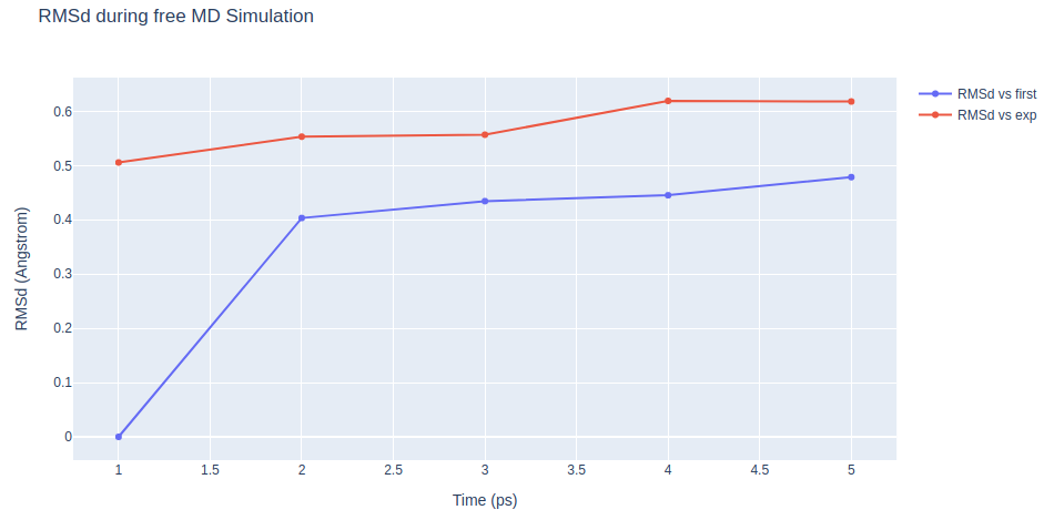
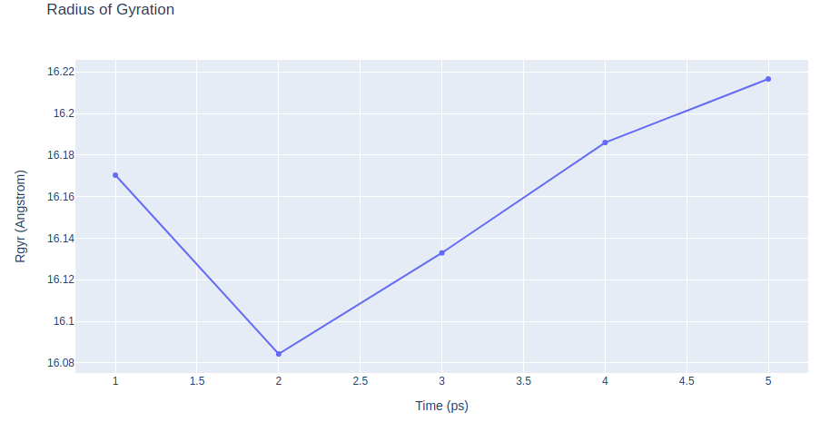
Step 2: Checking free MD simulation results
Checking results for the final step of the setup process, the free MD run. Plotting Root Mean Square deviation (RMSd) and Radius of Gyration (Rgyr) by time during the free MD run step. RMSd against the experimental structure (input structure of the pipeline) and against the minimized and equilibrated structure (output structure of the NPT equilibration step).
# cpptraj_rms: Computing Root Mean Square deviation to analyse structural stability
#              RMSd against minimized and equilibrated snapshot (backbone atoms)

# Import module
from biobb_analysis.ambertools.cpptraj_rms import cpptraj_rms

# Create prop dict and inputs/outputs
output_rms_first = pdbCode+'_rms_first.dat'

prop = {
    'mask': 'backbone',
    'reference': 'first'
}

# Create and launch bb
cpptraj_rms(input_top_path=output_ions_top_path,
            input_traj_path=output_free_traj_path,
            output_cpptraj_path=output_rms_first,
            properties=prop)
# cpptraj_rms: Computing Root Mean Square deviation to analyse structural stability
#              RMSd against experimental structure (backbone atoms)

# Import module
from biobb_analysis.ambertools.cpptraj_rms import cpptraj_rms

# Create prop dict and inputs/outputs
output_rms_exp = pdbCode+'_rms_exp.dat'

prop = {
    'mask': 'backbone',
    'reference': 'experimental'
}

# Create and launch bb
cpptraj_rms(input_top_path=output_ions_top_path,
            input_traj_path=output_free_traj_path,
            output_cpptraj_path=output_rms_exp,
            input_exp_path=output_pdb_path,
            properties=prop)
# Read RMS vs first snapshot data from file
with open(output_rms_first,'r') as rms_first_file:
    x,y = map(
        list,
        zip(*[
            (float(line.split()[0]),float(line.split()[1]))
            for line in rms_first_file
            if not line.startswith(("#","@"))
        ])
    )

# Read RMS vs experimental structure data from file
with open(output_rms_exp,'r') as rms_exp_file:
    x2,y2 = map(
        list,
        zip(*[
            (float(line.split()[0]),float(line.split()[1]))
            for line in rms_exp_file
            if not line.startswith(("#","@"))
        ])
    )

trace1 = go.Scatter(
    x = x,
    y = y,
    name = 'RMSd vs first'
)

trace2 = go.Scatter(
    x = x,
    y = y2,
    name = 'RMSd vs exp'
)

data = [trace1, trace2]

plotly.offline.init_notebook_mode(connected=True)

fig = {
    "data": data,
    "layout": go.Layout(title="RMSd during free MD Simulation",
                        xaxis=dict(title = "Time (ps)"),
                        yaxis=dict(title = "RMSd (Angstrom)")
                       )
}

plotly.offline.iplot(fig)
# cpptraj_rgyr: Computing Radius of Gyration to measure the protein compactness during the free MD simulation

# Import module
from biobb_analysis.ambertools.cpptraj_rgyr import cpptraj_rgyr

# Create prop dict and inputs/outputs
output_rgyr = pdbCode+'_rgyr.dat'

prop = {
    'mask': 'backbone'
}

# Create and launch bb
cpptraj_rgyr(input_top_path=output_ions_top_path,
            input_traj_path=output_free_traj_path,
            output_cpptraj_path=output_rgyr,
            properties=prop)
# Read Rgyr data from file
with open(output_rgyr,'r') as rgyr_file:
    x,y = map(
        list,
        zip(*[
            (float(line.split()[0]),float(line.split()[1]))
            for line in rgyr_file
            if not line.startswith(("#","@"))
        ])
    )

plotly.offline.init_notebook_mode(connected=True)

fig = {
    "data": [go.Scatter(x=x, y=y)],
    "layout": go.Layout(title="Radius of Gyration",
                        xaxis=dict(title = "Time (ps)"),
                        yaxis=dict(title = "Rgyr (Angstrom)")
                       )
}

plotly.offline.iplot(fig)
Post-processing and Visualizing resulting 3D trajectory
Post-processing and Visualizing the protein system MD setup resulting trajectory using NGL
Step 1: Imaging the resulting trajectory, stripping out water molecules and ions and correcting periodicity issues.
Step 2: Visualizing the imaged trajectory using the dry structure as a topology.
Building Blocks used:
cpptraj_image from biobb_analysis.cpptraj.cpptraj_image
Step 1: Imaging the resulting trajectory.
Stripping out water molecules and ions and correcting periodicity issues
# cpptraj_image: "Imaging" the resulting trajectory
#                Removing water molecules and ions from the resulting structure

# Import module
from biobb_analysis.ambertools.cpptraj_image import cpptraj_image

# Create prop dict and inputs/outputs
output_imaged_traj = pdbCode+'_imaged_traj.trr'

prop = {
    'mask': 'solute',
    'format': 'trr'
}

# Create and launch bb
cpptraj_image(input_top_path=output_ions_top_path,
            input_traj_path=output_free_traj_path,
            output_cpptraj_path=output_imaged_traj,
            properties=prop)
Step 2: Visualizing the generated dehydrated trajectory.
Using the imaged trajectory (output of the Post-processing step 1) with the dry structure (output of
# Show trajectory
view = nglview.show_simpletraj(nglview.SimpletrajTrajectory(output_imaged_traj, output_ambpdb_path), gui=True)
view.clear_representations()
view.add_representation('cartoon', color='sstruc')
view.add_representation('licorice', selection='JZ4', color='element', radius=1)
view

Output files
Important Output files generated:
structure.ions.pdb: System structure of the MD setup protocol. Structure generated during the MD setup and used in the MD simulation. With hydrogen atoms, solvent box and counterions.
sander.free.netcdf: Final trajectory of the MD setup protocol.
sander.free.rst: Final checkpoint file, with information about the state of the simulation. It can be used to restart or continue a MD simulation.
structure.ions.parmtop: Final topology of the MD system in AMBER Parm7 format.
Analysis (MD setup check) output files generated:
3htb_rms_first.dat: Root Mean Square deviation (RMSd) against minimized and equilibrated structure of the final free MD run step.
3htb_rms_exp.dat: Root Mean Square deviation (RMSd) against experimental structure of the final free MD run step.
3htb_rgyr.dat: Radius of Gyration of the final free MD run step of the setup pipeline.
Questions & Comments
Questions, issues, suggestions and comments are really welcome!
GitHub issues:
BioExcel forum: